Guidance, Navigation and Control. Personal project.

Steering a baseball into the strike zone with spin

A closed-loop 6-DOF GNC implementation for a pitched baseball. The ball carries one IMU and three reaction wheels, utilizing the magnus effect to steer. Over 0.45s of flight it estimates its state, solves for the spin that puts it on the target, and actuates itself onto that spin. Strike rate goes from 25% to 100%.

Demonstration

Run a single pitch comparing the GNC implementation with a normal pitch, using python in browser.

idle


Side view, height vs distance to plate
Catcher view, at the plate
n/aMiss to target [m]
n/aUncontrolled miss [m]
n/aCall
n/aFlight time [s]
n/aPeak |torque| [N·m]
n/aPosition error [m]

Summary

The aerodynamics

A 90mph fastball reaches the plate in under half a second. In that time the Magnus force can deflect the ball by more than a foot.

Spin is a usable control input with some limitations: the force is always perpendicular to velocity, its magnitude saturates with spin rate, and it can only change as fast as the angular momentum can be reoriented.

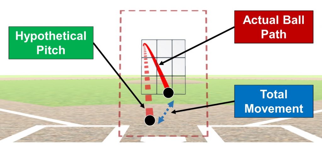
Diagram of pitch and the effect of ball aerodynamics.
Diagram of pitch movement due to aerodynamic effects.

Image source: American Baseball Coaches Association.

The strike zone

The target is a 0.432m by 0.55m box at a plane 16.8m from release. The ball either crosses inside it or it does not, which gives a clean terminal miss distance and a pass/fail metric. Guidance default aim is at the centre of the zone, but can be tuned.

The GNC

The point of the project was to write every layer of a GNC system myself rather than study them separately.

Target (x, z) at plate Guidance kinematic solve, 50Hz Control inner loop, 500Hz Plant 6-DOF, wheels, aero IMU gyro + accel EKF 11 states, 500Hz ω τ z = [gyro, accel]

Guidance never sees truth. It runs on the EKF estimate, and the EKF evaluates its onboard aerodynamic model at its own estimate.

Results

20 pitches with release dispersion in angle, speed, spin rate and release point. Each pitch is flown twice, once torque-free as a baseline and once under the full stack.

0.416 → 0.009mMedian miss to target46× reduction
25 → 100%Strike rate0.432 × 0.55m zone
0.536 → 0.069m90th-percentile missthe tail, not the median
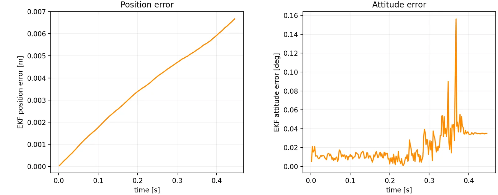
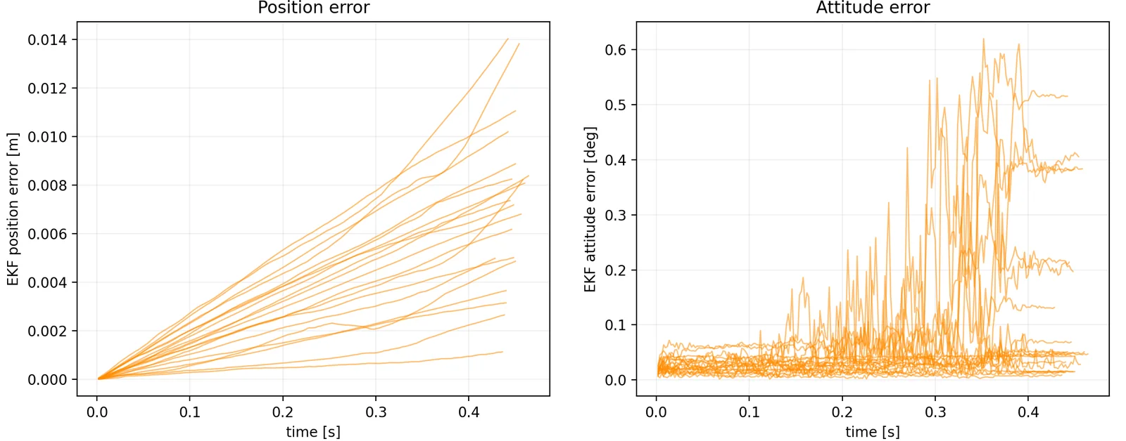
0.007mEKF terminal position errordead-reckoned, IMU only
Scope

The reaction wheels are not sized to a real motor. A 5N·m flywheel does not fit inside a baseball. That one component is idealised so the question under test is whether the estimator and the guidance law work. Mass properties, air density, drag and lift coefficients, sensor noise and bias, filter tuning and integration are all physical.

Dynamics and Physics

Motivation for choices
  • Spin drives ball trajectory: implement attitude dynamics with full quaternion 6-DOF physics.
  • Free flight with internal actuator: three reaction wheels.
  • Magnus effect is complex: use published aerodynamic models.
Methodology

State vector

13 physical states plus one speed per wheel $$ X = \begin{bmatrix} \mathbf{r} & \mathbf{v} & \mathbf{q} & \boldsymbol\omega & \boldsymbol\Omega \end{bmatrix} \in \mathbb{R}^{13+n} $$
  • $\mathbf r$, position (inertial frame).
  • $\mathbf v$, velocity (inertial frame).
  • $\mathbf q$, quaternion from body frame to inertial frame.
  • $\boldsymbol\omega$, angular rate (body frame).
  • $\boldsymbol\Omega$, speed of each reaction wheel about its own axis.

Aerodynamics

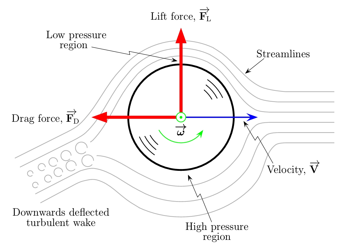
Simplified schematic of rotating ball aerodynamics with the Magnus effect.
Ball Aerodynamics. Simplified schematic of rotating ball aerodynamics with the Magnus effect.

Image source: Garry Robinson and Ian Robinson.

The aerodynamic model is based off a 2013 paper by Garry Robinson and Ian Robinson, The motion of an arbitrarily rotating spherical projectile and its application to ball games.

dynamic pressure, drag, Magnus lift $$ q = \tfrac12 \rho \lVert \mathbf v_i \rVert^2, \qquad \mathbf F_D = -\, q\, C_D A \, \hat{\mathbf v}, \qquad \mathbf F_L = q\, C_L(\omega)\, A \, \frac{\boldsymbol\omega_i \times \hat{\mathbf v}} {\lVert \boldsymbol\omega_i \times \hat{\mathbf v} \rVert} $$

Lift uses the inertial spin $\boldsymbol\omega_i = R(\mathbf q)\,\boldsymbol\omega_b$.

ω in rad/s $$ C_L(\omega) = 0.319\left(1 - e^{-2.48\times10^{-3}\,\omega}\right) $$

Invertible and saturating, so a required $C_L$ maps to a unique spin rate. Aerodynamic torque is zero; spin decay over 0.45s is negligible.

Rigid-body dynamics with wheels

angular momentum, attitude dynamics, translation $$ \mathbf L_b = J\,\boldsymbol\omega_b + A\,(I_w \odot \boldsymbol\Omega), \qquad \dot{\boldsymbol\omega}_b = J_{\text{eff}}^{-1} \left( \mathbf T_{\text{ext}} - A\,\boldsymbol\tau_w - \boldsymbol\omega_b \times \mathbf L_b \right) $$ $$ \dot{\boldsymbol\Omega} = \boldsymbol\tau_w \oslash I_w - A^{\mathsf T} \dot{\boldsymbol\omega}_b, \qquad \dot{\mathbf q} = \tfrac12\,\Xi(\mathbf q)\,\boldsymbol\omega_b, \qquad \dot{\mathbf v}_i = \mathbf g_i + \frac{\mathbf F_{\text{aero}}}{m} $$

Axes stacked in $A$, inertias $I_w$. $-A\boldsymbol\tau_w$ is the reaction: wheel torque hits the ball with the opposite sign.

Sensors

White noise plus a bias drawn once per flight. The accelerometer senses specific force, so gravity does not appear.

IMU measurement model $$ \mathbf z_g = \boldsymbol\omega_b + \mathbf b_g + \boldsymbol\eta_g, \qquad \mathbf z_a = R(\mathbf q)^{\mathsf T} \frac{\mathbf F_{\text{aero}}}{m} + \mathbf b_a + \boldsymbol\eta_a $$

It sees only the aerodynamic force, which does not depend on position.

Actuators

Three wheels, $I_w = 3\times10^{-6}\ \mathrm{kg\,m^2}$, saturated at $\pm 5\ \mathrm{N\,m}$.

Implementation
QuantityValueSource / note
Mass $m$0.145kgMLB regulation
Diameter0.074mMLB regulation
Inertia $I$0.4 m r²solid sphere
Air density $\rho$1.22kg/m³16°C, sea level
Drag coefficient $C_D$0.45constant over the Re band of a pitch
Max lift coefficient0.319saturating fit, spin-dependent
Release point16.8m, 1.8mdistance to plate, height
Nominal pitch90mph, 2200rpmbackspin about $-x$
Wheel inertia $I_w$3 × 10⁻⁶ kg m²3 orthogonal wheels
Torque limit±5N·midealised, not motor-sized
Gyro noise / bias1e-3 / 1e-4 rad/s1σ, bias drawn per flight
Accel noise / bias1e-3 / 1e-3 m/s²1σ, bias drawn per flight

Aero model validation

Flown with spin and spinless; the difference is the induced break.

PitchFlight [s]Horizontal [in]Vertical [in]Published range
4-seam fastball, 95mph / 2400rpm0.4240.0+14.9rise 15 to 17in
Curveball, 80mph / 2500rpm0.5040.0−15.5drop 10 to 15in
Slider, 85mph / 2400rpm0.47414.9−0.0horiz 6 to 15in
Gyro spin, 85mph / 2400rpm0.474−0.80.0no movement (control case)

Gyro spin producing no movement confirms the Magnus direction. $C_L$ ignores seam orientation, so two-seam is out of scope.

dynamics.pyState pack and unpack, quaternion kinematics and DCM, angular momentum, the state derivative, BallParams, and the drag and Magnus model with its $C_L$ fit and validation harness.
imu.py6-DOF IMU with per-flight bias draws.
run.pyScenario constants, DOP853 integration, terminal events, and the zero-order-hold GNC driver.

DOP853 throughout: $\text{rtol}=10^{-9}$ for the torque-free baseline, $10^{-8}$ across the zero-order-hold steps of a closed-loop flight. Plate and ground are terminal events.

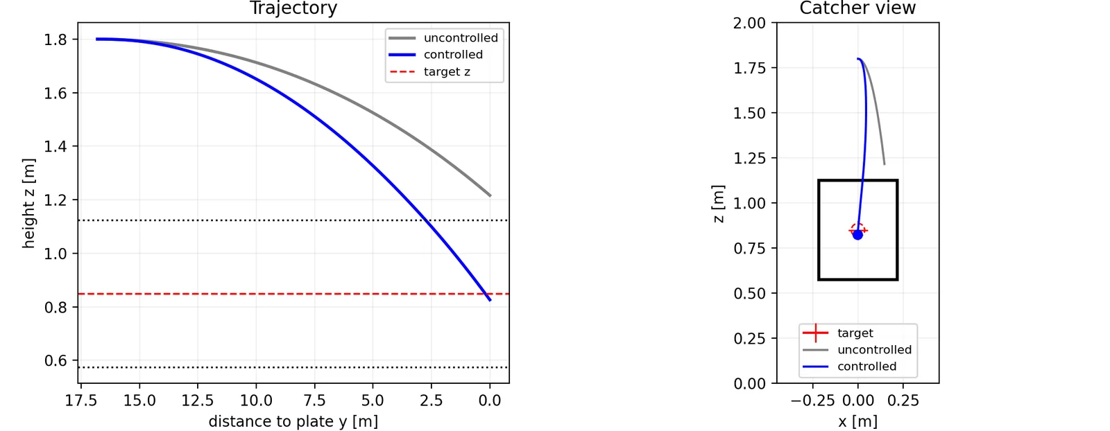
Two panels. Left: side view of height versus distance to the plate, with an uncontrolled trajectory arriving high above the target line and a controlled trajectory bending down onto it. Right: catcher's view showing the controlled pitch converging onto the target cross inside the strike zone box while the uncontrolled pitch ends above and right of the zone.
One nominal pitch. A 90mph fastball with 0.5° of yaw error. The baseline (grey) crosses 1.216m high and 0.147m wide, missing the target by 0.395m and the zone entirely; the controlled pitch (blue) crosses 0.024m from the target.

Guidance

Motivation for choices

Guidance turns a position error 16.8m away into a body-rate command, against a force perpendicular to velocity, saturating at $C_{L,\max}$, on a slew-limited axis. The law inverts the aerodynamics in closed form: no ODE solves, no Jacobians, no iteration.

Methodology

Each outer tick, from $(\hat{\mathbf r}, \hat{\mathbf v}, \hat{\mathbf q})$:

1. Time to go

Along-track speed is nearly constant.

$$ t_{\text{go}} = \frac{y_{\text{target}} - \hat y}{\hat v_y} $$

2. Required constant acceleration

Two-point boundary value problem.

$$ \mathbf a_{\text{req}} = \frac{2\left(\mathbf r_{\text{target}} - \hat{\mathbf r} - \hat{\mathbf v}\,t_{\text{go}}\right)}{t_{\text{go}}^2} $$

3. Remove what is not commanded

Gravity and drag act regardless.

$$ \mathbf a_{\text{cmd}} = \mathbf a_{\text{req}} - \mathbf g - \underbrace{\left(-\frac{ q\, C_D A}{m}\,\hat{\mathbf v}\right)}_{\text{drag}} $$

4. Project onto what Magnus can produce

The along-track part is unachievable.

$$ \mathbf a_\perp = \mathbf a_{\text{cmd}} - \hat{\mathbf v}\,\frac{\hat{\mathbf v}\cdot\mathbf a_{\text{cmd}}}{\lVert \hat{\mathbf v}\rVert^2} $$

5. Clip required lift coefficient

Magnus force set to $m\,\mathbf a_\perp$, clipped short of saturation.

$$ C_{L,\text{req}} = \min\!\left(\frac{m \lVert \mathbf a_\perp \rVert}{ q\,A},\; 0.99\,C_{L,\max}\right) $$

6. Invert the lift coefficient equation

Invert the $C_L$ aerodynamics from the physics section.

$$ \lVert\boldsymbol\omega_{\text{cmd}}\rVert = \frac{-\ln\!\left(1 - C_{L,\text{req}}/C_{L,\max}\right)}{2.48\times10^{-3}} $$

7. Calculate spin direction

Direction, from the Magnus cross product:

$$ \hat{\boldsymbol\omega}_{\text{cmd}} = \frac{\hat{\mathbf v}\times\mathbf a_\perp}{\lVert \hat{\mathbf v}\times\mathbf a_\perp \rVert} $$

8. Rotate into body axes

$$ \boldsymbol\omega_{\text{cmd}}^{b} = R(\hat{\mathbf q})^{\mathsf T}\,\boldsymbol\omega_{\text{cmd}}^{i} $$
Implementation

w_setpoint() in gnc.py: thirty lines, no solver, no state, 50Hz. The code calls the projected vector a_guid; it is $\mathbf a_\perp$ above.

# gnc.py, the guidance law in full
t_go = (target[1] - r_i[1]) / v_i[1]
if t_go < 0.09:                                       # terminal freeze
    return np.zeros(3), np.zeros(3), np.zeros(3)

a      = 2 * (target - r_i - v_i * t_go) / (t_go**2)    # required accel
a_cmd  = a - a_g - a_d                                  # strip gravity + drag
a_guid = a_cmd - v_i * np.dot(v_i, a_cmd) / v_norm2     # strip along-track

C_L_req  = min(np.linalg.norm(a_guid) * p.m / (q_dyn * p.area), C_L_max*.99)
w_cmd_i  = np.cross(v_i, a_guid) / v_norm2              # direction
w_cmd_i /= np.linalg.norm(w_cmd_i)
w_cmd_i *= -np.log(1 - C_L_req/C_L_max) / 2.48E-3       # invert C_L(w)

Known limitations

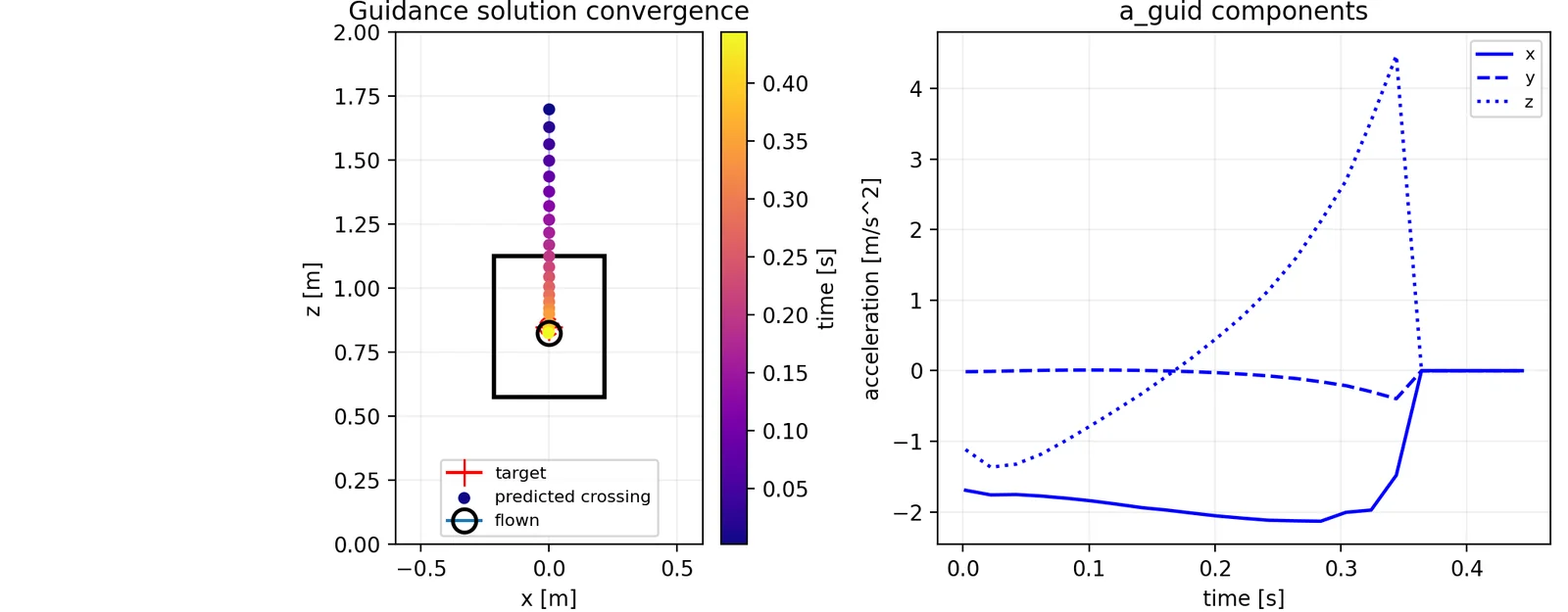
  • $1/t_{\text{go}}^2$ singularity. The solve blows up as $t_{\text{go}} \to 0$, so it is frozen below 0.09s and the last command is held. Wheel torque now peaks at 4.2 of 5N·m and never saturates.
  • Constant acceleration is approximate. Re-solving at 50Hz means it only holds 20ms at a time.
  • The axes differ. Vertical modulates backspin; lateral reorients the axis.
Two panels. Left: catcher view with the strike zone box, the target, and a colour-coded track of where each guidance solve predicts the ball will cross, walking down from 1.7 metres onto the target. Right: time histories of the three components of the guidance acceleration, with the vertical component rising to about 4.5 metres per second squared before dropping to zero.
The guidance solve converging. Each dot is one outer tick's prediction of the crossing point under $\mathbf a_\perp$, coloured by time. Early solves land short because Magnus cannot deliver the full $\mathbf a_{\text{cmd}}$; as flight time is spent the prediction walks onto the flown crossing (black ring). The drop to zero at 0.36s is the terminal freeze.

Control

Motivation for choices
  • Spin at 2200 rpm makes $\mathbf L$ large and cross coupled across axes.
  • $\mathbf L$ Coupling also resists change of spin direction: negate it from estimated states.
  • Aiming and slewing are different problems on different timescales: use zero-order hold on guidance commands.
Methodology

Cancel the gyroscopic coupling onto the wheel axes.

$$ \boldsymbol\tau_{\text{gyro}} = -A^{\mathsf T}\left(\boldsymbol\omega_b \times \mathbf L_b\right), \qquad \mathbf L_b = J\boldsymbol\omega_b + A(I_w \odot \boldsymbol\Omega) $$

Drive rate error to zero on a chosen time constant.

first-order rate loop, t_settle = 0.02s $$ \dot{\boldsymbol\omega}_{\text{des}} = \frac{\boldsymbol\omega_{\text{cmd}}^{b} - \boldsymbol\omega_b}{t_{\text{settle}}}, \qquad \boldsymbol\tau_{\text{fb}} = -A^{\mathsf T}\left(J_{\text{eff}}\,\dot{\boldsymbol\omega}_{\text{des}}\right) $$ $$ \boldsymbol\tau = \operatorname{clip}\!\left(\boldsymbol\tau_{\text{gyro}} + \boldsymbol\tau_{\text{fb}},\; \pm\tau_{\max}\right) $$

Rates

Inner loop and EKF at 500Hz, guidance at 50Hz. The 10:1 separation lets guidance treat the inner loop as instantaneous. Torque is zero-order-hold.

inner_loop() in gnc.py.

# gnc.py, the inner loop in full
L_b       = p.J @ w_b + p.A @ (p.I_w * Om)      # wheel momentum included
tau_gyro  = -p.A.T @ np.cross(w_b, L_b)         # cancel the cross coupling

w_dot_des = (w_cmd_b - w_b) / t_settle          # first-order error decay
tau_fb    = -p.A.T @ (p.J_eff @ w_dot_des)      # torque that produces it

tau = np.clip(tau_gyro + tau_fb, -p.tau_limit, p.tau_limit)
Four panels. The first three show body rate about x, y and z: a stepped commanded setpoint in red, the achieved rate in blue, and truth as a black dotted line lying on top of the achieved rate. The fourth shows three wheel torques oscillating within plus and minus five newton-metres, peaking near four late in flight without touching the limits.
Inner loop tracking. Achieved rate (blue) against the 50Hz commanded setpoint (red) and truth (dotted). The loop tracks the step of each outer tick within its 0.02s time constant; truth and the estimate are indistinguishable at this scale. Torque peaks at 4.2N·m and never reaches the ±5N·m limit.

Monte Carlo

Motivation for choices
  • Dispersion comes from release conditions, the variation a pitcher cannot remove. Position offset is the hardest: a pure bias that has to be flown out.
  • Vertical and lateral miss are reported separately; the axes are not equally hard.
  • Release dispersion is drawn from a single RandomState(4000); each trial's IMU biases and EKF initialisation are seeded from its index. The whole campaign reproduces exactly.
Methodology

20 pitches. Dispersion, 1σ:

  • Release angle 0.25° in yaw and pitch.
  • Speed 1.5mph, spin rate 100rpm.
  • Release point 0.1m in both $x$ and $z$.

Per trial:

  1. Draw the dispersion from the trial's seeded generator.
  2. Fly the baseline: torque-free, DOP853.
  3. Fly it again closed-loop: fresh IMU biases, fresh EKF from a perturbed estimate.
  4. Terminate at the plate or the ground; record the crossing.
Implementation
MetricUncontrolledEKF + kinematic GNCNote
Combined miss, median0.416m0.009mdistance to target at the plate
Combined miss, p900.536m0.069mthe tail
Vertical $|\Delta z|$, median0.402m0.007mmodulate existing backspin
Vertical $|\Delta z|$, p900.526m0.063m
Lateral $|\Delta x|$, median0.074m0.004mreorient the spin axis
Lateral $|\Delta x|$, p900.195m0.026m
Crossing spread $\sigma_z$0.133m0.026mdispersion, not bias
Crossing spread $\sigma_x$0.122m0.023m
Strike rate25%100%inside the 0.432 × 0.55m box
Peak wheel torque, mediann/a1.83 of 5N·mno saturation on any trial
Terminal EKF position error, mediann/a0.007mdead-reckoned, IMU only
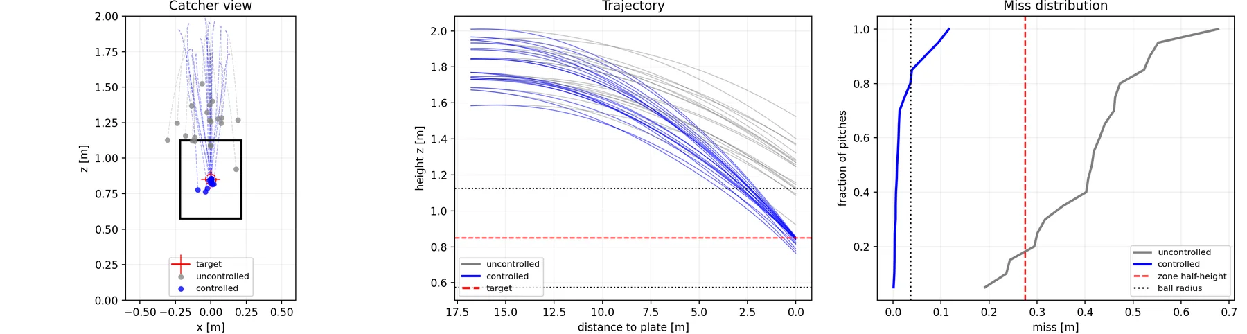
Three-panel Monte Carlo figure. Left: catcher-view scatter of crossing points, with grey uncontrolled points scattered above and around the strike zone box and blue controlled points collapsed into a tight cluster on the target. Middle: a bundle of twenty trajectory pairs, the grey ones arriving high and the blue ones converging on the target line at the plate. Right: cumulative miss distributions, the controlled curve reaching one hundred percent below 0.12 metres while the uncontrolled curve stretches out past 0.6 metres.
20 dispersed pitches. The uncontrolled (grey) scatters outside the zone; the controlled (blue) aligns onto the target. In the miss distribution every controlled pitch lands inside 0.12m, against a spread reaching 0.68m uncontrolled.

Results

  • Controlled pitches perform significantly better. Every controlled pitch lands closer to the target than any of the uncontrolled pitches. 25% strike rate to 100% strike rate.
  • Spin is not tracked mid-flight. The setpoint steps every 20ms and the ball is slew-limited, so the commanded and achieved rates only agree in the mean. It does not matter: what reaches the plate is the integral of the force, not the instantaneous rate.
  • Navigation is the same order as the miss. Median EKF error at the plate is 0.007m against a median miss of 0.009m. Guidance tuning alone will not go much further; the dead-reckoned position is the floor.