Soft Checksums: OOD Detection for Scientific ML

Demonstration

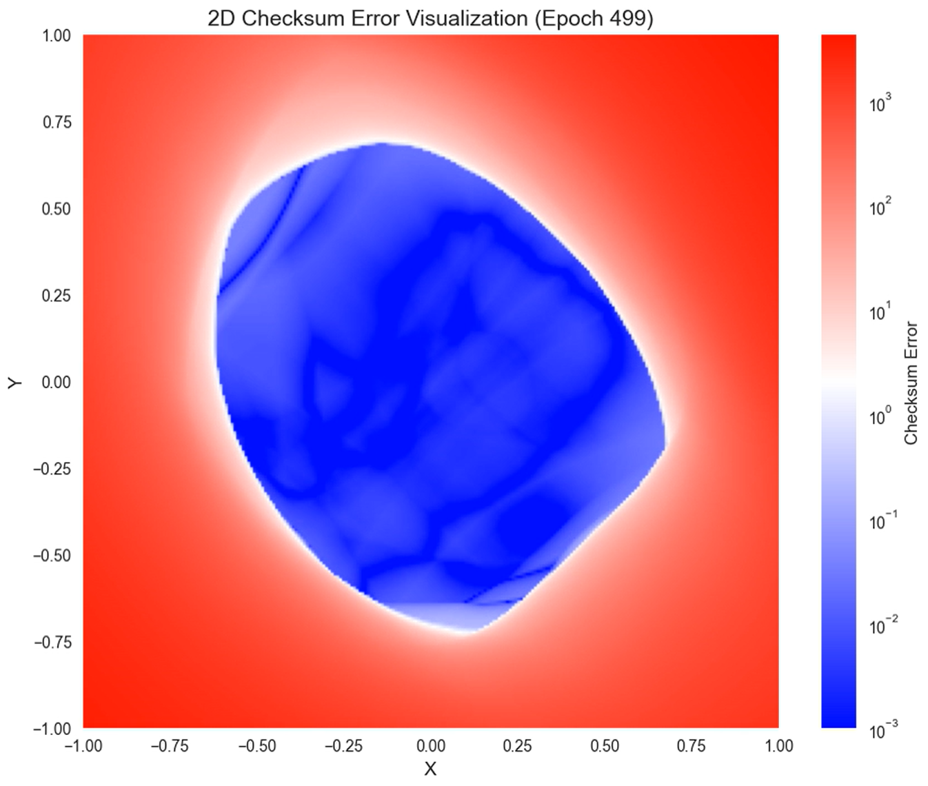
This runs the actual trained sum-checksum model in your browser with Pyodide and NumPy. Load it, then move the query point around the 2D toy domain. Inside the in-distribution disk the three predicted outputs stay consistent with the checknode, so the checksum error stays low; drag outside and the predictions break down and the error explodes. The domain, the three outputs, and this error map are the setup described in the Toy Problem section below.

summation checksum · width 256 · depth 2 idle

Query point x₁ 0.10

Query point x₂ 0.05

Flag threshold ε 0.20

Checksum error over the input domain (trained model)

Output	True f(x)	Model ŷ
y₁ = sin x₁ + cos x₂	–	–
y₂ = x₁ · x₂	–	–
y₃ = e^{−(x₁²+x₂²)}	–	–

the checksum, computed in the model's normalized output space

load the model to compute the checksum

–Checksum error |C − Ĉ|

–Prediction error (MSE)

–Verdict

The heatmap is the trained model's checksum error across the domain (blue = low, in-distribution; red = high, out-of-distribution), evaluated live in NumPy on a grid. Table outputs are shown in real units (de-normalized); the checksum itself is computed on the model's normalized outputs, which is what the checknode is trained against, so its terms differ from the real-unit values.

Summary

The problem

Surrogate models train on expensive physics simulations to provide fast approximations. However, standard regression models output point estimates without built-in confidence metrics or error bounds. If given an input outside their training space, they still return a concrete value without signaling uncertainty.

Detecting these out-of-distribution (OOD) points prevents invalid estimates from propagating through larger engineering workflows. Established approaches like deep ensembles, Monte Carlo dropout, and Bayesian neural networks provide uncertainty metrics, but require running multiple inference passes or training separate models.

The idea

This method adapts checksum principles from data communication. An extra output node (the checknode) is added to the network and trained to predict a deterministic function of the primary outputs, such as their sum. For in-distribution inputs, the checknode closely matches the computed sum, keeping the checksum error low. On unfamiliar inputs, the checknode and primary outputs extrapolate differently, causing the checksum error to spike. This discrepancy functions as an OOD flag produced directly within a single forward pass.

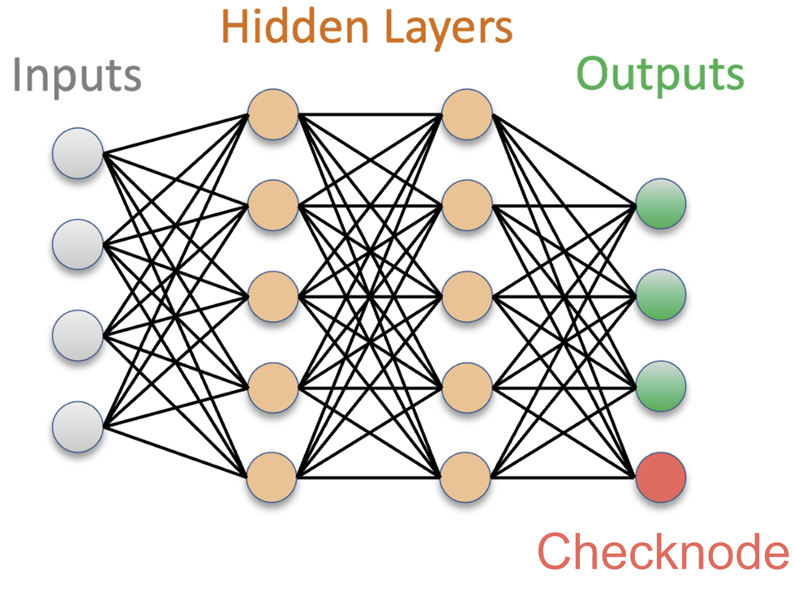
A fully connected neural network with grey input nodes, three orange hidden layers, three green regular output nodes, and one red output node at the bottom labelled Checknode. — **The checknode.** A standard regression network with an added output node. The green nodes represent standard predictions, while the red checknode outputs an estimate of the checksum over those predictions.

Results

Evaluated on a 0D auto-ignition combustion dataset (with in-distribution defined as peak temperatures below 2500 K), the tuned sine checksum clearly separates ID from OOD points while preserving baseline regression accuracy.

99.66%AUROC, tuned sine checksum0.5 is a coin flip, 1.0 is perfect

97.7 → 0.05%Missed OOD at the 99% thresholdbefore → after the checksum loss

1 passAdded inference costcompared to N-model ensembles

4 termsComposite lossprediction + loss + penalty + reward

Computational cost

Because the checksum function operates strictly on the model's outputs rather than intermediate weights or inputs, the score requires no auxiliary models, sampling passes, or calibrated distance metrics. The computational overhead is limited to evaluating one extra node and a final difference calculation.

Background

Design motivation

Surrogate networks require dependable reliability indicators to avoid silent failures on unseen input regimes.
Unlike classification models with probability distributions, standard regression offers no native uncertainty metric.
Uncertainty estimation must remain computationally lightweight to run within real-time simulation pipelines.

Methodology

When a surrogate fails

Consider a simple 1D example: a network trained to approximate $$y=x$$ on the interval $$0. Outside this interval ($x\ge 3$), the network extrapolates poorly and fails to indicate that it is operating outside its training bounds.$

Piecewise target function (x ≥ 3 unobserved) $$ y = \begin{cases} x & \text{if } x < 3 \\ 3 & \text{if } x \ge 3 \end{cases} $$

In general, bare regression outputs cannot distinguish valid interpolations from untrustworthy extrapolations.

Existing OOD detection

Standard methods quantify uncertainty through repeated evaluation or ensemble sampling. Bayesian neural networks sample from learned weight distributions, Monte Carlo dropout aggregates multiple stochastic forward passes, and deep ensembles measure variance across several distinct models. While effective, these techniques multiply training and inference overhead. In classification, methods such as Outlier Exposure and energy-based models structure training so the network explicitly responds differently to out-of-distribution inputs. We apply a similar philosophy to regression without adding inference passes.

Checksums

First formalized for serial data transmission by Fletcher in 1982, checksums append verification bytes so receivers can detect data corruption through consistency checks. Traditional checksums are binary (matching or failing), which is impractical for regression models that inherently carry small residual errors. The soft checksum instead uses the continuous magnitude of the mismatch between the predicted checknode and the computed output function as a graded OOD metric.

Method

Design motivation

The checksum function operates solely on output variables, generalizing across regression tasks without adding input-space complexity.
The functional form must be straightforward to optimize while sufficiently constrained so that the network cannot trivially satisfy it during extrapolation.
Passive training is insufficient: the network must be explicitly regularized to produce inconsistent checknode values on OOD samples to prevent smooth extrapolation.

Methodology

Augmenting the network

For a regression network mapping inputs to outputs, $\hat{\mathbf y} = \hat f(\mathbf x;\,\boldsymbol\theta)$ , the output layer is expanded by one node to produce both the target predictions and an estimated checksum $\hat{\mathbb C}_y$ .

one network, outputs plus a checknode $$ \left(\hat{\mathbf y},\; \hat{\mathbb C}_y\right) = \hat f(\mathbf x;\,\boldsymbol\theta) $$

The checksum function and error

The checksum function $\mathbb C$ is a fixed, deterministic mapping over the predicted outputs. While a simple sum provides a straightforward baseline, composing the sum with a sine function introduces nonlinearity that improves sensitivity. The checksum error is defined as the absolute difference between the checknode output and the evaluated checksum function.

summation and sine checksum functions $$ \mathbb C(\mathbf y) = \sum_i y_i, \qquad \mathbb C(\mathbf y) = \sin\!\left(\omega \left| \sum_i y_i \right|\right) $$

checksum error: predicted checknode vs. function of outputs $$ \epsilon_{\mathbb C} = \left| \mathbb C(\hat{\mathbf y}) - \hat{\mathbb C}_y \right| $$

Because $\mathbb C$ requires only the model outputs, this metric can be computed directly at inference time without reference labels.

A four-part loss

Training optimizes a multi-objective loss function. The primary term is standard mean-squared error (MSE) on the physical target predictions.

prediction loss (MSE) $$ \mathcal L_{\text{MSE}}(\mathbf y, \hat{\mathbf y}) = \frac1n \sum_{i=1}^{k} (y_i - \hat y_i)^2 $$

The checksum loss $(\alpha)$ fits the checknode to the checksum of the ground-truth targets, while the checksum penalty $(\beta)$ penalizes discrepancies between the checknode and the predicted outputs to maintain internal consistency across the training distribution.

checksum loss and checksum penalty $$ \mathcal L_{\text{loss}} = \frac{\alpha}{k}\left(\mathbb C(\mathbf y) - \hat{\mathbb C}_y\right)^2, \qquad \mathcal L_{\text{pen}} = \frac{\beta}{k}\left(\mathbb C(\hat{\mathbf y}) - \hat{\mathbb C}_y\right)^2 $$

On out-of-distribution samples, the checksum reward $(\gamma)$ encourages discrepancy between the checknode and the predicted checksum. A reciprocal formulation bounded by $\kappa$ and stabilized by $\mu$ prevents gradient instability once separation is established.

checksum reward on OOD samples (saturating) $$ \mathcal L_{\text{rew}} = \gamma \,\min\!\left(\kappa,\; \left[\left(\mathbb C(\hat{\mathbf y}_{\text{OOD}}) - \hat{\mathbb C}_y\right)^2 + \mu\right]^{-1}\right) $$

total loss driving backpropagation $$ \mathcal L_{\text{total}} = \mathcal L_{\text{MSE}} + \mathcal L_{\text{loss}} + \mathcal L_{\text{pen}} + \mathcal L_{\text{rew}} $$

Implementation

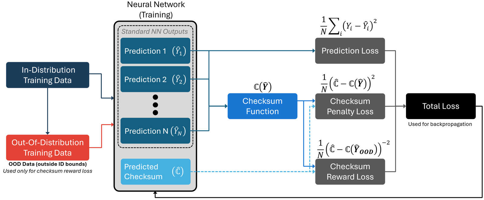
In-distribution data flows through the prediction, checksum loss, and penalty terms; generated OOD data is routed strictly through the reward term. The losses sum into a single scalar for backpropagation.

Training data flow diagram. In-distribution and out-of-distribution training data enter a neural network whose outputs are predictions plus a predicted checksum. The predictions feed a prediction loss and a checksum function; the checksum function and checknode feed a checksum penalty loss and a checksum reward loss. All losses sum into a total loss used for backpropagation. — **Training data flow.** In-distribution samples drive prediction accuracy and consistency terms, while synthetic out-of-distribution samples drive the reward term.

Term	Weight	Data	Objective
Prediction (MSE)	1.0	ID	Fits the surrogate to target data
Checksum loss	α	ID	Aligns checknode with ground-truth checksum
Checksum penalty	β	ID	Enforces consistency between predictions and checknode
Checksum reward	γ	OOD	Maximizes output discrepancy on OOD points

OOD Generation

Design motivation

The reward loss requires representative OOD samples during training, though empirical out-of-distribution data is rarely known in advance.
To remain domain-agnostic, synthetic generation must rely strictly on the bounding envelope of the training set.
Generating samples both near the distribution boundaries and further into the domain helps the detector establish clear decision margins.

Methodology

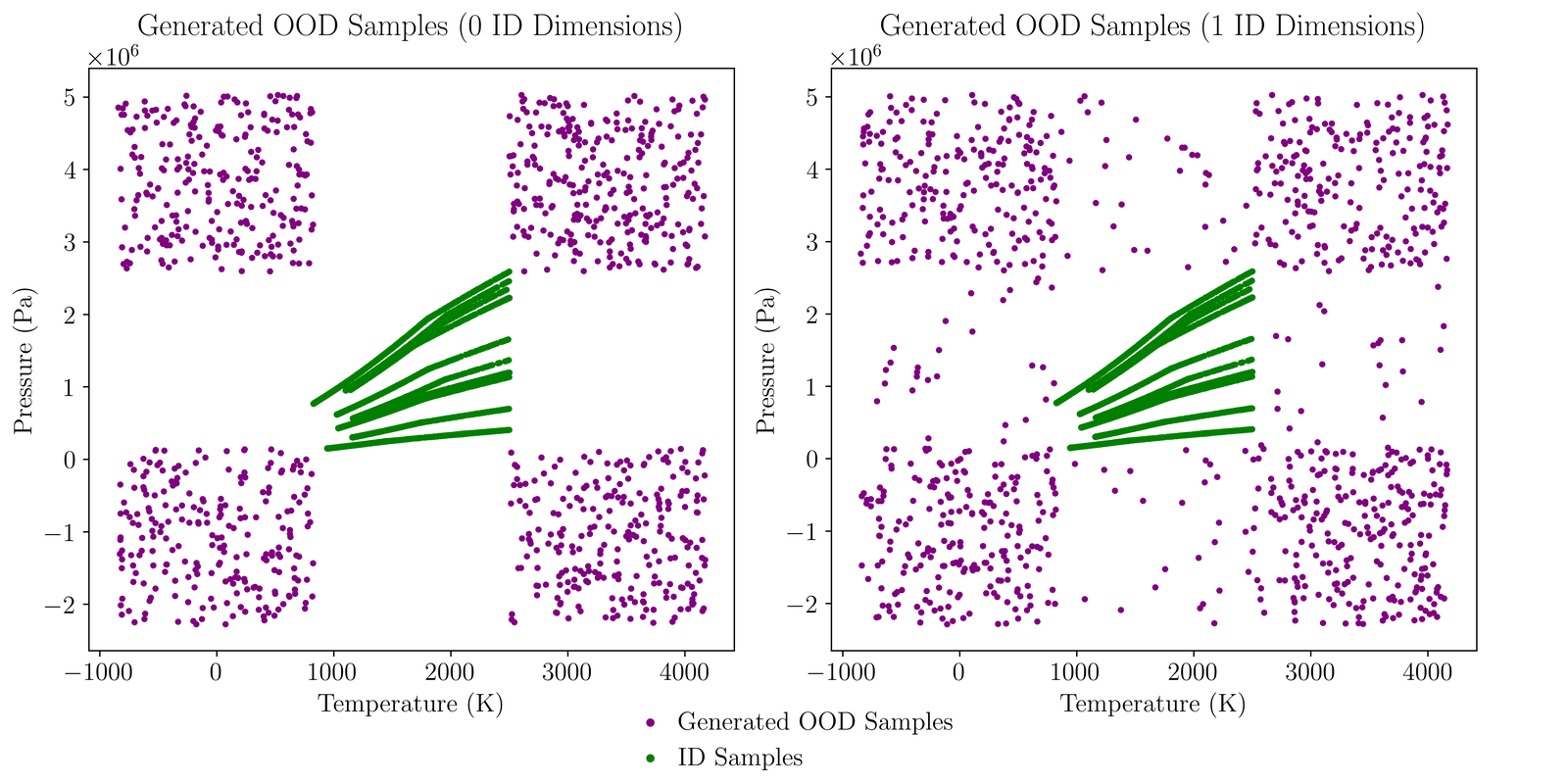
OOD samples are synthesized on the fly from the training data envelope. For each generated point, a subset of input dimensions is sampled outside the observed $[\min,\max]$ range while remaining dimensions stay within range. An ID Max parameter controls how many dimensions may remain in-distribution: forcing every dimension out produces corner points far from the distribution, while allowing some dimensions to stay in range seeds points along the immediate decision boundary.

Implementation

Two scatter plots of pressure versus temperature. Green ID samples form a diagonal band in the centre. Purple generated OOD samples fill the surrounding space: on the left, clustered in four corner blocks away from the data; on the right, also bordering the ID band directly. — **Synthetic OOD sampling.** Green indicates ID data; purple indicates generated OOD points. **Left:** all dimensions forced out of range, placing samples in distal corners. **Right:** select dimensions permitted within range, generating points directly along the distribution boundary.

Synthetic OOD points are used solely within the reward loss calculation; they do not enter the prediction or penalty loss terms.

Toy Problem

Design motivation

A 2D toy problem allows direct visualization of the error surface across the entire domain. Evaluating the network on a uniform grid clarifies how the checksum response relates to input distance from the training manifold. You can explore this exact error surface, output by output, in the interactive demonstration at the top of the page.

Methodology

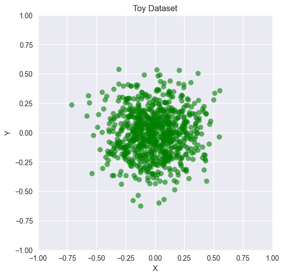
The in-distribution dataset is defined as a cluster of 2D points near the origin. Each point maps to three distinct functional outputs (periodic, multiplicative, and radial decay) to ensure the checksum does not exploit trivial linear relationships.

three toy outputs from one 2D input $$ y_1 = \sin(x_1) + \cos(x_2), \qquad y_2 = x_1 x_2, \qquad y_3 = e^{-(x_1^2 + x_2^2)} $$

Scatter plot of green training points clustered around the origin within roughly plus or minus 0.5 in both axes. — **In-distribution dataset.** A compact cluster of training points sampled near the origin.

Heatmap of checksum error over the 2D input domain. A blue low-error island covers the in-distribution region in the middle; error rises sharply to red across the surrounding out-of-distribution area, on a logarithmic colour scale. — **In-distribution dataset.** A compact cluster of training points sampled near the origin.

Implementation

Evaluating the model across the domain $x_1, x_2 \in [-1, 1]$ shows that checksum error correlates closely with actual prediction error on a log-log scale. As prediction error increases in extrapolation regions, the checksum error rises proportionally without requiring access to true reference labels.

Results

Evaluation objectives

Validation requires evaluating realistic physical simulations where out-of-distribution inputs pose genuine failure risks.
Ablation experiments test combinations of loss weights to isolate the impact of each term against an unregularized baseline network.
Performance is assessed primarily through AUROC and false negative rates, alongside surrogate regression accuracy.

Methodology

The combustion dataset

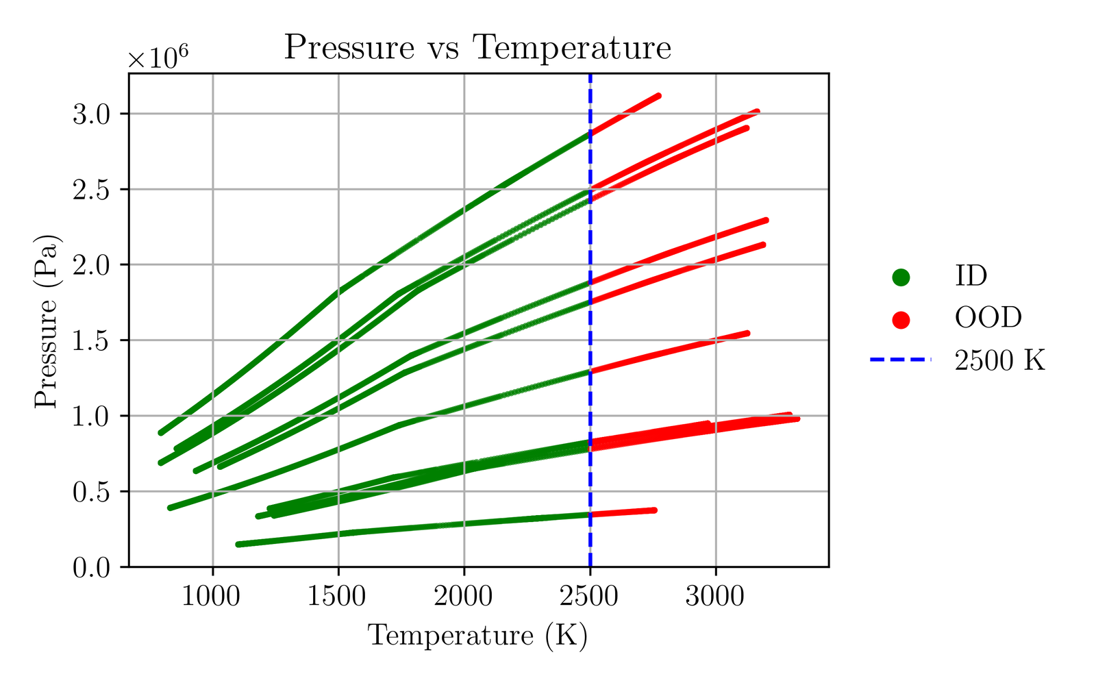
The benchmark is a 0D auto-ignition combustion problem solved with Cantera. Seven chemical species ( $C_2H_4,\ O_2,\ H_2,\ CO,\ CO_2,\ H_2O$ and inert $$N_2$$ ) interact across three primary reaction pathways. The surrogate model predicts net species production rates $\omega$ from temperature, pressure, and composition. Trajectories with peak temperatures below 2500 K constitute in-distribution data, while hotter states are withheld as out-of-distribution targets.

Scatter of pressure versus temperature. Several green in-distribution trajectory bands rise from low temperature up to a dashed vertical line at 2500 K, beyond which the same trajectories continue in red as out-of-distribution. — **Dataset partitioning.** Ignition trajectories in pressure-temperature space. Green samples are in-distribution; trajectories exceeding the 2500 K boundary (dashed line) are withheld as OOD validation points.

Network architecture: 3 hidden layers (256 units each), learning rate $10^{-4}$ , batch size 256, 1500 epochs. All reported values represent five-run averages to account for weight initialization variance.

Implementation

Performance metrics

FNR (95% / 99%): False negative rate, measuring the percentage of OOD samples that fall below the 95th or 99th percentile of in-distribution error (lower is better).
AUROC: Area under the receiver operating characteristic curve, representing the probability of ranking a random OOD sample above a random ID sample (higher is better).
ID error: Mean squared error on in-distribution test samples, verifying that checksum regularization does not degrade baseline regression performance (lower is better).

Performance comparison

Configuration	FNR 99% ↓	AUROC ↑	ID error ↓	Note
Baseline, summation (α,β,γ = 0)	56.98%	87.86%	3.07×10⁻⁴	Untrained checknode
Baseline, sine (α,β,γ = 0)	90.17%	60.16%	2.86×10⁻⁵	No separation signal
Summation, α = 1, γ = 1	5.51%	98.74%	7.16×10⁻⁵	Low-complexity configuration
Sine, α = 1 (loss only)	1.88%	99.65%	1.11×10⁻⁴	Lowest false negative rate
Sine, α = 1, γ = 1	1.89%	99.66%	1.02×10⁻⁴	Highest overall AUROC

Best values per column are highlighted in blue. The summation checksum offers consistent baseline accuracy with low implementation complexity, whereas the sine checksum achieves higher detection sensitivity at a slight trade-off in in-distribution error stability. The complete eight-weight ablation is detailed in the full paper.

Error distribution analysis

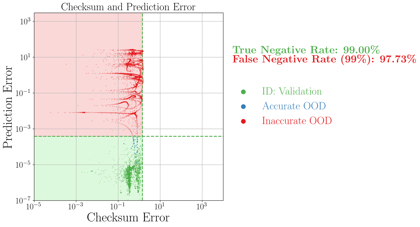
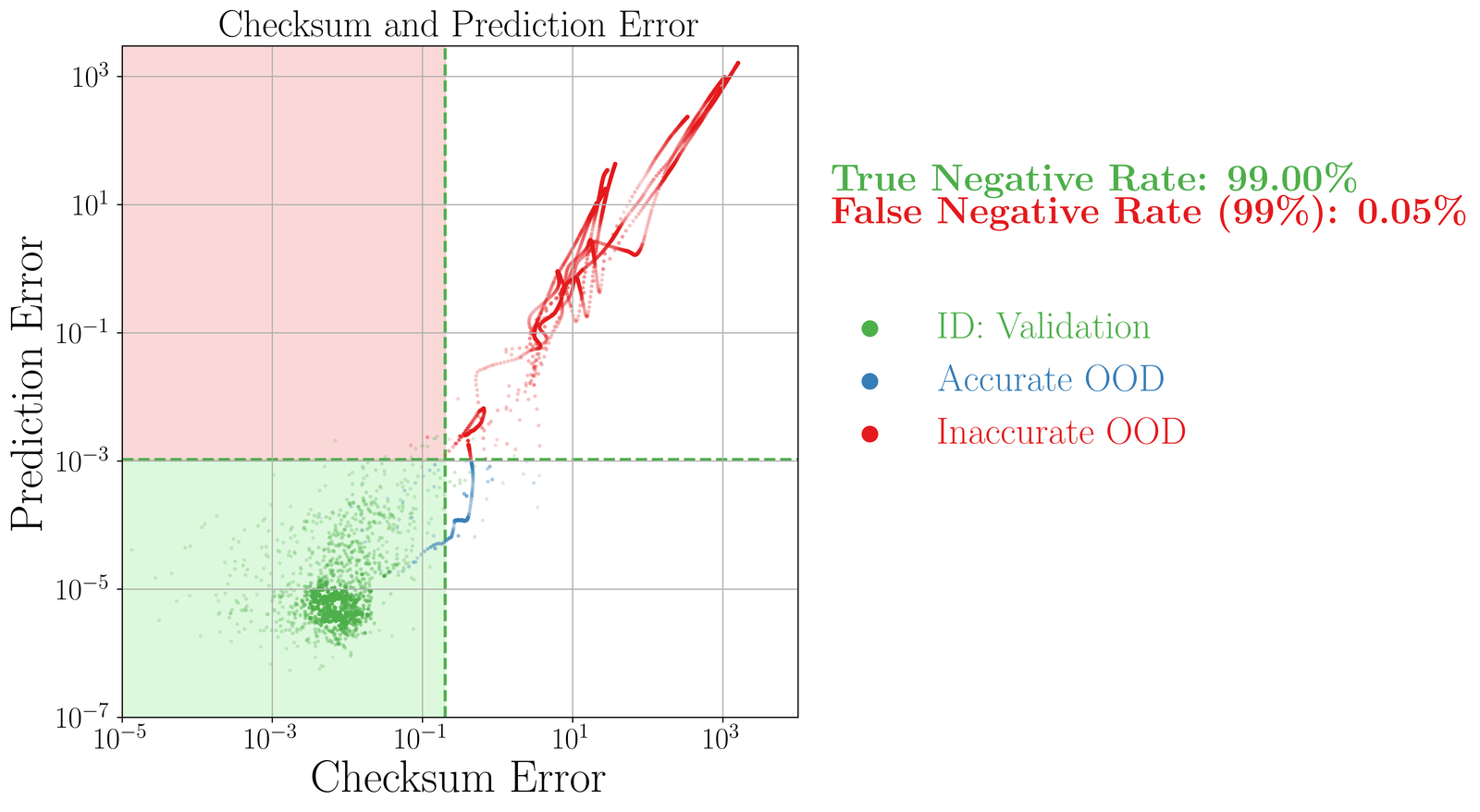
Plotting checksum error against prediction error highlights the impact of the loss formulation. In an effective detector, OOD points exhibit elevated checksum error alongside prediction error. Without checksum training, the errors remain uncorrelated; incorporating the loss and reward terms aligns them along a clear diagonal, isolating OOD cases.

Scatter of prediction error versus checksum error on log axes. Green in-distribution points sit low-left; red inaccurate OOD points are stacked in a vertical column at a similar checksum error, giving no diagonal relationship. Annotation: false negative rate 97.73%. — **Baseline (no checksum loss).** Checksum and prediction error are uncorrelated; 97.7% of OOD samples fall below the detection threshold.

The same axes after training with checksum loss and reward. Green ID points cluster low-left; blue and red OOD points climb along a clear diagonal to the upper right. Annotation: false negative rate 0.05%. — **Baseline (no checksum loss).** Checksum and prediction error are uncorrelated; 97.7% of OOD samples fall below the detection threshold.

Green points represent in-distribution validation data, red points indicate inaccurate OOD predictions, and blue points denote accurate OOD predictions. The green bounding box marks the accepted region, while the red box highlights unflagged predictions with high error. Checksum training significantly reduces false acceptances in the critical upper-left region.

Inference workflow

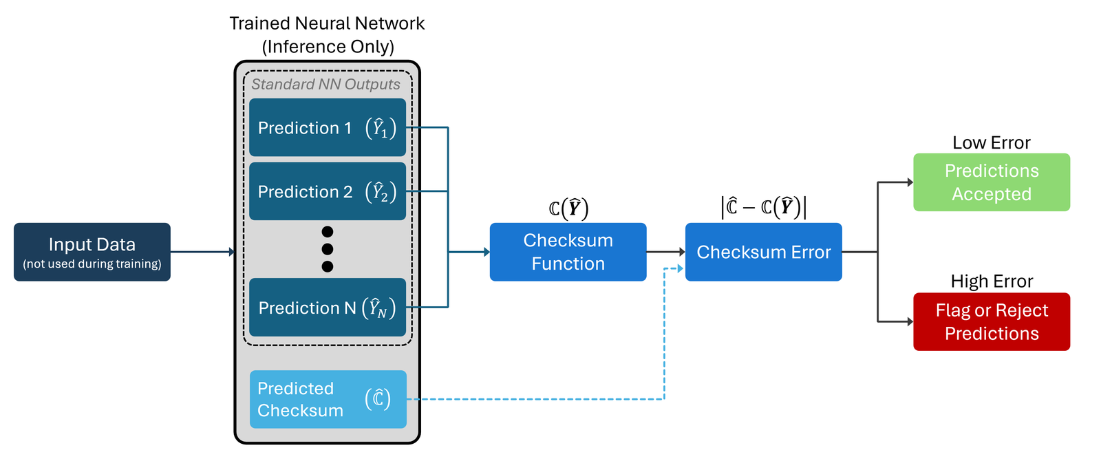
During inference, evaluation requires only a single forward pass. The network computes target predictions and the checknode simultaneously, after which the checksum function is evaluated. If the calculated difference remains below the threshold, the prediction is accepted; if it exceeds the threshold, the sample is flagged for review or routed to a full physics simulation.

Inference flow diagram. Input data enters a trained network producing predictions and a predicted checksum. A checksum function and a checksum error block compare them; low error routes to a green Predictions Accepted box, high error to a red Flag or Reject Predictions box. — **Inference execution.** A single forward pass yields target outputs and the checknode. Discrepancies between the predicted checknode and the evaluated checksum determine acceptance or escalation.

Scope and limitations

The in-distribution threshold here is defined by a fixed temperature cutoff (2500 K), which creates a clear benchmark but simplifies boundary definitions found in more complex domains. While the sine checksum provides higher detection sensitivity, the summation checksum offers a more stable baseline for tasks prioritizing raw regression precision. Future work will benchmark these configurations directly against deep ensembles and MC dropout, test alternative nonlinear checksum functions, and evaluate multi-node verification architectures.